
Each chapter so far took one tool at a time. Real work runs them in a row: pandas loads and cleans a table, NumPy turns it into , scikit-learn sets a baseline, PyTorch tries to beat it, and Matplotlib shows whether it did. This chapter runs that pipeline once, end to end. It adds no new library, only the habits that keep a pipeline’s numbers honest.
The data is 400 made-up training jobs: memory, size and sequence length, and whether the job ran out of memory. The memory a job needs grows with size times sequence length, a curve no straight line follows. Each panel below is a value its line really made, from the table to the two scores.
import numpy as npimport pandas as pdimport torchfrom torch import nnfrom sklearn.linear_model import LogisticRegressionfrom sklearn.model_selection import train_test_splittorch.manual_seed(0)df = pd.read_csv('data/oom.csv')df = df.dropna()df['oom'] = (df['oom'] == 'yes').astype(int)X = df[['mem_gb', 'batch_size', 'seq_len']].to_numpy(dtype=np.float32)y = df['oom'].to_numpy()X_train, X_test, y_train, y_test = train_test_split(X, y, test_size=0.25, random_state=0)mean, std = X_train.mean(axis=0), X_train.std(axis=0)X_train, X_test = (X_train - mean) / std, (X_test - mean) / stdbaseline = LogisticRegression().fit(X_train, y_train)base_acc = baseline.score(X_test, y_test)Xt, yt = torch.from_numpy(X_train), torch.from_numpy(y_train)model = nn.Sequential(nn.Linear(3, 16), nn.ReLU(), nn.Linear(16, 2))loss_fn = nn.CrossEntropyLoss()optimizer = torch.optim.AdamW(model.parameters(), lr=0.05)loss_fn(model(Xt), yt)for epoch in range(300): optimizer.zero_grad() loss = loss_fn(model(Xt), yt) loss.backward() optimizer.step()model.eval()with torch.no_grad(): pred = model(torch.from_numpy(X_test)).argmax(dim=1)mlp_acc = (pred.numpy() == y_test).mean().item(){'baseline': round(base_acc, 3), 'mlp': round(mlp_acc, 3)}df.shape
(400, 4)
df.head(4)
| mem_gb | batch_size | seq_len | oom | |
|---|---|---|---|---|
| 0 | 16 | 64 | 2048.0 | yes |
| 1 | 16 | 8 | 1024.0 | yes |
| 2 | 80 | 64 | 256.0 | no |
| 3 | 24 | 4 | 2048.0 | no |
One row per training job, and whether it ran out of GPU memory. seq_len reads as floats: it has blanks, and NaN is a float.
Each stage hands the next one a known . gives a , drops the 14 jobs with no sequence length, and makes a float32 . The and standard deviation come from the training rows alone, and applies them to both halves, so nothing leaks from the .
the baseline first. draws one straight boundary and gets 0.866 of the test jobs right, where answering “no” to every job gets 0.577. The small network, , and again, can bend its boundary, and after 300 it gets 0.969 of the same rows right. Without the baseline, 0.969 would be a number with nothing to compare it to.
import matplotlib.pyplot as plt
# y_test, base_acc and mlp_acc are the stepper's: the same seeded run.
# Always answering "no" is the floor any model must beat.
scores = {
    'always "no"': (y_test == 0).mean().item(),
    'logistic regression': base_acc,
    'MLP': mlp_acc,
}
fig, ax = plt.subplots(figsize=(6, 2.6), layout='constrained')
bars = ax.barh(list(scores), list(scores.values()))
ax.bar_label(bars, fmt='%.3f', padding=4)
ax.margins(x=0.15)
ax.invert_yaxis()
ax.set_xlabel(f'accuracy on the {len(y_test)} test jobs')
ax.set_title('Same rows, three answers')
fig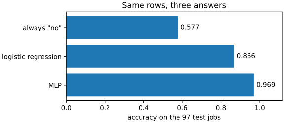
Print the after every stage: one line shows what the stage did. An goes further and stops the run at the first that’s wrong, printing the one it got.
import pandas as pd
df = pd.read_csv('data/oom.csv').dropna()
X = df[['mem_gb', 'batch_size', 'seq_len']].to_numpy()
# Double brackets select a one-column table, not a Series.
y = df[['oom']].to_numpy()
# Print the shapes after each stage.
X.shape, y.shape((386, 3), (386, 1))# Or assert them: the run stops at the first one that's wrong.
assert X.shape == (len(df), 3), X.shape
assert y.shape == (len(df),), y.shapeAssertionError: (386, 1)This is where most people slip. Double brackets make a one-column table, so its is (386, 1), not (386,), and not every library says so. it with only a warning, raises, and it against a model’s 1-D output into a wrong with a warning. The catches it in all three.
Randomness enters in several places: the split, the starting weights, the shuffle. each one (random_state=0, torch.manual_seed(0)) and a re-run prints the same numbers, so a change in the score comes from a change in the code. PyTorch doesn’t promise the same numbers across releases, platforms, or CPU and , and some operations vary run to run unless you call torch.use_deterministic_algorithms(True).
import torch
from torch import nn
def first_layer(seed):
    torch.manual_seed(seed)
    return nn.Linear(3, 2).weight
# The same seed draws the same starting weights; another seed doesn't.
torch.equal(first_layer(0), first_layer(0))Truetorch.equal(first_layer(0), first_layer(1))FalseTime a slow stage before you change it. reads a clock, and the difference between two readings is the time in between. In a , runs one line many times and prints the and its spread.
import time

start = time.perf_counter()
model = train_model(X_train, y_train)
print(f'training took {time.perf_counter() - start:.2f} s')
Explore in a : run a cell, look, change it. Its cells keep their variables and can run in any order, so it can show a result no top-to-bottom run gives. Once the pipeline works, move it into a : python pipeline.py runs top to bottom in a fresh process every time.
The habit this chapter adds: make every run say where it stands, with a baseline to beat, the after each stage, and a so the same code prints the same numbers.
Homework
The packet is the whole pipeline on this chapter’s jobs, one tested stage at a time: load and clean the table, make the with the right and scale them without a leak, a baseline that must score at least 80%, train a model that must reach 93%, and save the comparison as a PNG. A last function runs all five in a row, and the model must beat the baseline.
Chapter 10 workbook
Unzip, follow the README once to set up, then run pytest until it's green.
What you now know
Every term the course has taught, under the chapter that first used it. Select one for its definition.